
A dimensional hierarchy is set of related data tables that align to different levels (see Figure 3.19). The tables commonly have one‐to‐many or many‐to‐one relationships with each other.
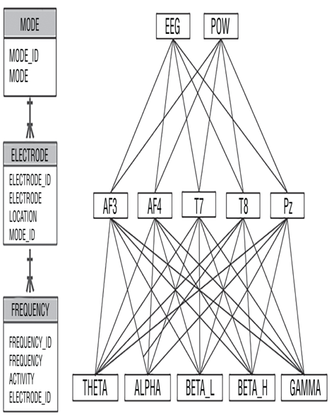
FIGUER 3.19 A dimensional hierarchy
The hierarchy shown in Figure 3.19 could be named the “brainjammer dimension.” The frequencies roll up to electrodes, and the electrodes roll up to modes. This hierarchical representation of data provides two benefits. The first benefit is that it reduces the complexity of a fact table. If the mode, electrode, and frequency of the reading were all stored on a single fact table, it would be difficult to deduce the relationship between those columns. When represented by the dimensional hierarchy, this is not the case. The second benefit is the hierarchy provides the means for drilling up and down into the data, where drilling up renders summarized data and drilling down renders more details. If you want to see which mode a reading or group of readings is generated from, you can drill up to find that.
Design a Solution for Temporal Data
The concept of temporal data is structured around the need to know the data stored in a table within a specific timeframe, instead of what is stored in the table now. Explained in another way, if you want to know the value stored in the LOCATION column on 2021‐01‐19, a date in the past, you can use a temporal data solution. The following snippet shows how to create a temporal table:
CREATE TABLE [dbo].[ELECTRODE]([ELECTRODE_ID] INT NOT NULL IDENTITY(1,1) PRIMARY KEY CLUSTERED,[ELECTRODE] NVARCHAR (50) NOT NULL,[LOCATION] NVARCHAR (50) NOT NULL,[SYSSTARTTIME] DATETIME2 GENERATED ALWAYS AS ROW START NOTNULL,[SYSENDTIME] DATETIME2 GENERATED ALWAYS AS ROW END NOT NULL,PERIOD FOR SYSTEM_TIME (SYSSTARTTIME, SYSENDTIME))
WITH (SYSTEM_VERSIONING = ON)
When executed on a SQL database, this SQL creates a table referred to as a system‐versioned table. This SQL query also creates another table to store data history. The insertion of a row into the ELECTRODE table results in the following:
+————–+———–+————+————–+————+
| ELECTRODE_ID | ELECTRODE | LOCATION | SYSSTARTTIME |SYSENDTIME|
+————–+———–+————+————–+————+
| 1 | AF3 | Front Left | 2022-01-19 | 9999-12-31 |
| … | … | … | … | … |
+————–+———–+————+————–+————+
No row is inserted into the history (the temporal table) until the original data is updated. The values for SYSSTARTTIME and SYSENDTIME are generated by the system. Notice the default value for an empty datetime is in the SYSENDTIME column.
The following SQL query updates the AF3 electrode:
UPDATE ELECTRODE
SET ELECTRODE = ‘AF3i’, LOCATION = ‘Top Left’
WHERE ELECTRODE_ID = 1
This query results in the updating of the data on the ELECTRODE table, which is system‐versioned, as expected. The value in the SYSENDTIME column remains empty, as the row contains the most current data.
+————–+———–+————+————–+————+
| ELECTRODE_ID | ELECTRODE | LOCATION | SYSSTARTTIME |SYSENDTIME|
+————–+———–+————+————–+————+
| 1 | AF3i | Top Left | 2022-01-19 | 9999-12-31 |
+————–+———–+————+————–+————+
Performing a SELECT query on the temporal table results in the following:
+————–+———–+————+————–+————+
| ELECTRODE_ID | ELECTRODE | LOCATION | SYSSTARTTIME |SYSENDTIME|
+————–+———–+————+————–+————+
| 1 | AF3 | Front Left | 2022-01-19 | 2022-01-19 |
+————–+———–+————+————–+————+
Figure 3.20 illustrates how the table looks when you use Azure Data Studio to query the database.
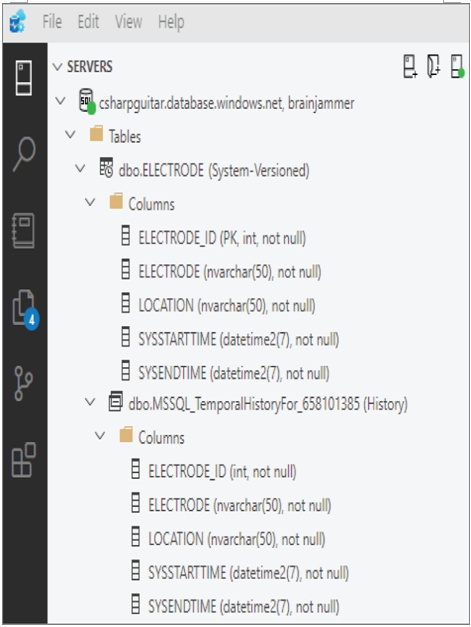
FIGUER 3.20 A temporal tableEach time a row is updated, the system generates a row in the history table to show its previous values. At any time you are required to perform historical analysis, then you have a place to retrieve the values (the dimensional values) that were current at a given time.